|
|
| Table of Contents | Back to Lecture 3: Tangent Vectors and the Tangent Space | On to Lecture 5: Tensor Fields |
Question How are the local coordinates of a given tangent vector for one chart related to those for another?
Answer Again, we use the chain rule. The formula
|
|
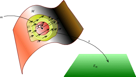
In other words, a tangent vector through a point m in M is a collection of n numbers (local coordinates) Vi = dxi/dt (specified for each chart x at m) where the quantities for one chart are related to those for another according to the formula
v | i |
= |   ixj ixj |
vj |
This leads to the following definition.
Definition 4.1 A contravariant vector at m  M is a collection vi of n quantities (defined for each chart at m) which transform according to the formula M is a collection vi of n quantities (defined for each chart at m) which transform according to the formula
It follows that contravariant vectors "are" just tangent vectors: the contravariant vector vi corresponds to the tangent vector given by so we shall henceforth refer to tangent vectors and contravariant vectors. A contravariant vector field V on M associates with each chart x a collection of n smooth real-valued coordinate functions Vi of the n variables (x1, x2, . . . , xn), such that evaluating Vi at any point gives a vector at that point. Further, the domain of the Vi is the whole of the range of x. Similarly, a contravariant vector field V on U |
The tranformation rule for all contravariant vector fields is therefore given as follows.
|
Contravariant Vector Transformation Rule
|
where now the Vi are functions of the associated coordinates (x1, x2, . . . , xn), and similarly for the barred coordinates. Note that the transformation rule is only valid on the intersection of the images of x and .
Notes 4.2
1.The above formula is reminiscent of matrix multiplication: In fact, let  be the matrix whose ij th entry is
  i/xj, then the above equation becomes, in matrix form:
V |
= | D |
V. |
where we think of V and  as column vectors.
2. By "transform," we mean that the above relationship holds between the coordinate functions Vi of the xi associated with the chart x, and the functions i of the i, associated with the chart .
3. Note the formal symbol cancellation: if we cancel the 's, the x's, and the superscripts on the right, we are left with the symbols on the left!
4. From the proof of 3.6, we saw that, if V is any smooth contravariant vector field on M, then
| V = Vi | xi | . |
at t = 0. Thus this vector has coordinate functions
dt |
= | Fi, |
which are the same as the original coordinates. In other words, the tangent vectors are "the same" as ordinary vectors in En.
(b) An Important Local Vector Field Recall from Example 3.4 (e) the definition of the vectors /xi: At each point m in a manifold M, we have the n vectors /x1, /x2, . . . , /xn, where the typical vector /xi was obtained by taking the derivative of the path:
| xi |
= | vector obtained by differentiating the path xj = |
|
, |
where the constants are chosen to make xi(t0) correspond to m for some t0. This gave
| xi | j |
= |  ij ij | . |
Now, there is nothing to stop us from defining n different vector fields /x1, /x2, . . . , /xn, in exactly the same way: at each point in the coordinate neighborhood of the chart x, associate the vector above.
Note: /xi is a field, and not the i th coordinate of a field. Its jth local coordinate under the chart x is given by ij = xj/xi at every point in the image of x.
Question Since the coordinates do not depend on x, does it mean that the vector field is constant?
Answer No. Remember that a tangent filed is a field on (part of) a manifold, and as such, it is not, in general, constant. The only thing that is constant are its coordinates under the specific chart x. The corresponding coordinates under another chart are j/xi (which are not constant in general).
Question What does the vector field /xi look like?
Answer Click here to see.
(c)
Patching Together Local Vector Fields
The vector field in the above example has the disadvantage that is local. We can "extend" it to the whole of M by making it zero near the boundary of the coordinate patch, as follows. If m M and x is any chart of M, lat x(m) = y and let D be a disc or some radius r centered at y entirely contained in the image of x. Now define a vector field on the whole of M by
|
where
| R = | r - |x(p) - y|) |
The fact that the local coordinates vary smoothly with p M now follows from the fact that all the partial derivatives of all orders vanish as you leave the domain of x. Note that this field agrees with /xi at the point m.
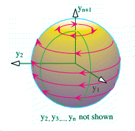
(d) (Based on Example 3.2(c)) Take M = Sn, with stereographic projection given by the two charts discussed earlier (Example 2.3(f) in Lecture 2). Consider the circulating vector field on Sn defined at the point y = (y1, y2, . . . , yn, yn+1) by the paths
 (y1cost - y2sint, y1sint + y2cost, y3, ... , yn+1).
(For fixed y = (y1, y2, . . . , yn, yn+1) this defines a path at the point y -- see Example 3.2(c).) This is a circulating field in the y1y2-plane. (See the figure. Note: the length of the tangent vector at a given point equals the radius of the latitutde circle on which it sits.)
Question What are its local coordinates under the two charts x and associated with stereographic projection?
Answer We saw in Lecture 2 that
|
so | V1 | = |
|
= |
|
= | -x2 | |||||||||||||
|
so | V2 | = |
|
= |
|
= | x1 | |||||||||||||
|
so | V3 | = |
|
= | 0 | |||||||||||||||
| ... | |||||||||||||||||||||
|
so | Vn | = |
|
= | 0 |
|
so | 1 | = |
|
= |
|
= | -2 |
|||||||||||||
|
so | 2 | = |
|
= |
|
= | 1 |
|||||||||||||
|
so | 3 | = |
|
= | 0 | |||||||||||||||
| ... | |||||||||||||||||||||
|
so | n | = |
|
= | 0 |
Thus, the local coordinates are given by
V = [-x2, x1, 0, 0, ... , 0] , and
= [-2, 1, 0, 0, ... , 0]
Question I don't believe that they transform according to the transformation rule for contravariant vectors!
Answer They do. Click here for the interesting details.
We now look at the gradient. If  is a smooth scalar field on M, and if x is a chart, then we obtain the locally defined vector field /xi. By the chain rule, these functions transform as follows:
| i |
= | xj |
xji | , |
or, writing Cj = /xj and  i = /i,
| i | = | Cj | xji | . |
This leads to the following definition.
|
Definition 4.4 A covariant vector field C on M associates with each chart x a collection of n smooth functions Ci(x1, x2, . . . , xn) which satisfy:
Covariant Vector Transformation Rule
|
Notes 4.5
1. If D is the matrix whose ij th entry is xi/j, then the above equation becomes, in matrix form:
C | = | CD |
where now we think of C and as row vectors.
2. Note that
| (D)ij |
= | xik |
kxj |
= | xixj |
= | ji |
, |
and similarly for D. Thus, and D are inverses of each other.
3. Note again the formal symbol cancellation: if we cancel the 's, the x's, and the superscripts on the right, we are left with the symbols on the left!
4. Guide to memory: In the contravariant objects, the barred x goes on top; in covariant vectors, on the bottom. In both cases, the non-barred indices match.
Note From now on, all scalar and vector fields are assumed smooth.
Question Geometrically, a contravariant vector is a vector that is tangent to the manifold. How do we think of a covariant vector?
Answer The key to the answer is this:
Definition 4.6 A smooth 1-form, or a smooth cotangent vector field on the manifold M (or on an open subset U of M) is a function F that assigns to each tangent vector field V on M (or on the subset U) a scalar field F(V) which is smooth (in the sense that F converts smooth vector fields to smooth scalar functions)., and which has the following properties:
F(  V) = F(V). V) = F(V).
for every pair of tangent vector fields V and W, and every scalar |
|
Proposition 4.7 (Covariant Fields are One-Form Fields)
There is a one-to-one correspondence between covariant vector fields on M (or U) and 1-forms on M (or U). Thus, we can think of covariant tangent fields as nothing more than 1-forms. |
Examples 4.8
(a) Let M = S1 with the charts:
= arg(-z) discussed in Lecture 2. There, we saw that the change-of-coordinate maps, are given by
| x | = |
|
| = |
| , |
with
/x = x/ = 1,
so that the change-of-coordinates do nothing. It follows that functions C and specify a covariant vector field iff C = . (Then they are automatically a contravariant field as well.) For example, let
().
This field circulates around S1. On the other hand, we could define
() = - sin = sin x.
This field is illustrated in the following figure.
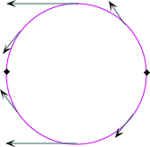
(The length of the vector at the point ei is given by sin .)
(b) Let be a scalar field. Its ambient gradient, grad , is given by
| grad = |
|
along V is given by V. grad . (If V happens to be a unit vector at some point, then this is the directional derivative at that point.) In other words, dotting with grad assigns to each contravariant vector field the scalar field F(v) = V. grad which tells it how fast is changing along V. We also get the 1-form identities:
V) = F(V).
The coordinates of the corresponding covariant vector field are
| F(/xi) |
= | (/xi).grad |
|||||||||||||||||||||||
| = |
|
||||||||||||||||||||||||
| = | xi | , |
which is the example that first motivated the definition.
(c) Generalizing (b), let  be any smooth vector field in Es defined on an open set containing M itself. Then the operation of dotting with is a linear function from smooth tangent fields on M to smooth scalar fields. Thus, by the proof of Proposition 4.7, it is a cotangent field on M with local coordinates given by applying the linear function to the canonical charts /xi:
| Ci | = | xi |
. | |
The gradient is an example of this, since we are taking
= 
in the preceding example.
Note that dotting with depends only on the tangent component of . This leads us to the (very important!) next example.
(d) If V is any tangent (contravariant) field, then we can appeal to (c) above and obtain an associated covariant field. The coordinates of this field are not the same as those of V. To find them, we write:
| V | = | Vi | xi |
(See Note 4.2 (4).) |
Hence, the local coordinates are
| Cj | = | xj |
. | V | = | Vi | xj |
. | xi |
Question The vectors /xi are mutually orthogonal, so that the last dot product is just ij, right?
Answer Wrong! The tangent vectors /xi are not necessarily orthogonal in general (look at the picture of these fields from earlier in this lecture) , so the dot products don't behave as simply as we might suspect.
Instead, we can define certain functions gij by
| gij | = | xi |
. | xj |
so that
gives the correct relation between the coordinates of a covariant vector and the corresponding contravariant vector field. (Note how the indices cancel to leave us with a lowered index...) We shall see the quantities gij again presently. One last thing:
Definition 4.9 If V and W are contravariant (or covariant) vector fields on M, and if is a real number, we can define new fields V+W and V by
and ( V)i = Vi.
It is easily verified that the resulting quantities are again contravariant (or covariant) fields. |
These operations turn the set of all smooth contravariant (or covariant) fields on M into a vector space. Note that we cannot expect to obtain a vector field by adding a covariant field to a contravariant field.
1. Suppose that Xj is a contravariant vector field on the manifold M with the following property: at every point m of M, there exists a local coordinate system xi at m with Xj(x1, x2, . . . , xn) = 0. Show that Xi is identically zero in any coordinate system.
2. Give and example of a contravariant vector field that is not covariant. Justify your claim.
3. Verify the following claim If V and W are contravariant (or covariant) vector fields on M, and if is a real number, then V+W and V are again contravariant (or covariant) vector fields on M.
4. Verify the following claim in the proof of Proposition 4.7: If Ci is covariant and Vj is contravariant, then CkVk is a scalar.
5. Let : SnE1 be the scalar field defined by (p1, p2, . . . , pn+1) = pn+1.
(a) Express as a function of the xi and as a function of the j.
(b) Calculate Ci = / xi and j = /j.
(c) Verify that Ci and C-j transform according to the covariant vector transformation rules.
6. Is it true that the quantities xi themselves form a contravariant vector field? Prove or give a counterexample.
7. Prove that  and
and  in Proposition 4.7 are inverse functions.
8. Prove: Every covariant vector field is of the type given in Example 4.8(d). That is, obtained from the dot product with some contrravariant field.
| Table of Contents | Back to Lecture 3: Tangent Vectors and the Tangent Space | On to Lecture 5: Tensor Fields |
 M is defined in the same way, but its domain is restricted to x(U).
 +
+