In the last lecture, we saw how the scalar product in E_s gave rise to a type (0, 2) covariant tensor field g_ij. Here, we generalize this concept.

Definition 6.1 A smooth inner product on a manifold M is a function -,- that associates to each pair of smooth contravariant vector fields X and Y a scalar (field) X, Y , satisfying the following properties. symmetry:   X, Y = Y, X for all X and Y, bilinearity: aX, bY = ab X, Y for all X and Y, and scalars a and b X, Y+Z = X, Y + X, Z X+Y, Z = X, Z + Y, Z . non-degeneracy:   If X, Y = 0 for every Y, then X = 0. We also call such a gizmo a symmetric bilinear form. A manifold endowed with a smooth inner product is called a Riemannian manifold.

Before we look at some examples, let us see how these things can be specified. First, notice that, if x is any chart, and p is any point in the domain of x, then

X, Y

=

XiYj

xi

,

xj

This gives us smooth functions

gij

=

xi

,

xj

such that

X, Y = g_ijXⁱY^j

and which, by Proposition 5.3, constitute the coefficients of a type (0, 2) symmetric tensor. We call this tensor the fundamental tensor or metric tensor of the Riemannian manifold.

Examples 6.2

(a) Take M = E_n, with the usual inner product; we find g_ij = _ij.

(b) (Minkowski Metric) M = E₄, with g_ij given by the matrix

G

=

1 0 0 0 0 1 0 0 0 0 1 0 0 0 0 -c2 ,

where c is the speed of light.

Question How does this effect the length of vectors?
Answer We saw in Lecture 3 that, in E_n, we could think of tangent vectors in the usual way; as directed line segments starting at the origin. The role that the metric plays is that it tells you the length of a vector; in other words, it gives you a new distance formula:

Euclidean 3- space: d(x, y) = [(y₁ - x₁)² + (y₂ - x₂)² + (y₃ - x₃)²]^1/2
Minkowski 4-space: d(x, y) = [(y₁ - x₁)² + (y₂ - x₂)² + (y₃ - x₃)² - c²(y₄ - x₄)²]^1/2

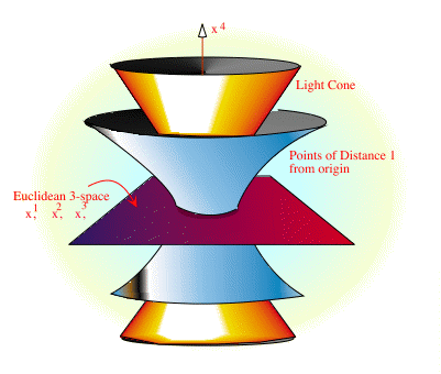
Geometrically, the set of all points in Euclidean 3-space at a distance r from the origin (or any other point) is a sphere of radius r. In Minkowski space, it is a hyperbolic surface. In Euclidean space, the set of all points a distance of 0 from the origin is just a single point; in M, it is a cone, called the light cone. (See the figure.)

Minkowski 4-Space

(c) If M is any manifold embedded in E_s, then we have seen above that M inherits the structure of a Riemannian metric from a given inner product on E_s. In particular, if M is any 3-dimensional manifold embedded in E₄ with the metric shown above, then M inherits such a inner product.

(d) As a particular example of (c), let us calculate the metric of the two-sphere M = S², with radius r, using polar coordinates x¹ = , x² = . To find the coordinates of g_** we need to calculate the inner product of the basis vectors /x¹, /x² in the ambient space E_s. We saw in Section 3 that the ambient coordinates of /xⁱ are given by

j th coordinate

=

yj xi

where

y₁ = r sin(x¹) cos(x²)
y₂ = r sin(x¹) sin(x²)
y₃ = r cos(x¹)

Thus,

x1	=	r(cos(x1)cos(x2), cos(x1)sin(x2), -sin(x1))
x2	=	r(-sin(x1)sin(x2), sin(x1)cos(x2), 0)

This gives

g₁₁ = /x¹, /x¹ = r²
g₂₂ = /x², /x² = r² sin²(x¹)
g₁₂ = /x¹,/x² = 0,

so that

g**

=

r2 0 0 r2sin2 (x1) .

(e) The n-Dimensional Sphere Let M be the n-sphere of radius r with generalized polar coordinates.

y₁ = r cos x¹
y₂ = r sin x¹ cos x²
y₃ = r sin x¹ sin x² cos x³
  ...
y_n-1 = r sin x¹ sin x² sin x³ sin x⁴ ... cos x^n-1
y_n = r sin x¹ sin x² sin x³ sin x⁴ ... sin x^n-1 cos xⁿ
y_n+1 = r sin x¹ sin x² sin x³ sin x⁴ ... sin x^n-1 sin xⁿ.

(Notice that x¹ is playing the role of and the x², x³, . . . , x^n-1 the role of .) Following the line of reasoning in the previous example, we have

x1	=	(-r sin x1, r cos x1 cos x2, r cos x1 sin x2 cos x3 , ... , r cos x1 sin x2... sin xn-1 cos xn, r cos x1 sin x2 ... sin xn-1 sin xn)
x2	=	(0, -r sin x1 sin x2, . . . , r sin x1 cos x2 sin x3... sin xn-1 cos xn, r sin x1 cos x2 sin x3 ... sin xn-1 sin xn)
x3	=	0, 0, -r sin x1 sin x2 sin x3, r sin x1 sin x2 cos x3 cos x4 . . . , r sin x1 sin x2 cos x3 sin x4... sin xn-1 cos xn, r sin x1 sin x2 cos x3 sin x4 ... sin xn-1 sin xn)

and so on. This gives

g₁₁ = /x¹, /x¹ = r²
g₂₂ = /x², /x² = r²sin²x¹
g₃₃ = /x³, /x³ = r²sin²x¹ sin² x²
 ...
g_nn = /xⁿ, /xⁿ = r²sin²x¹ sin² x² ... sin² x^n-1
g_ij = 0 if i j

so that

g**

=

r2 0 0 ... 0 0 r2sin2x1 0 ... 0 0 0 r2sin2x1 sin2 x2 ... 0 ... ... ... ... ... 0 0 0 ... r2sin2x1 sin2 x2 ... sin2 xn-1 .

(f) Diagonalizing the Metric Let G be the matrix of g_** in some local coordinate system, evaluated at some point p on a Riemannian manifold. Since G is symmetric, it follows from linear algebra that there is an invertible matrix P = (P_ji) such that

PGPT

=

±1 0 0 0 0 ±1 0 0 ... ... ... ... 0 0 0 ±1

at the point p. Let us call the sequence (±1,±1, . . . , ±1) the signature of the metric at p. (Thus, in particular, the Minkowski metric has signature (1, 1, 1, -1).) If we now define new coordinates ^j by

xⁱ = P_ji^j,

ij

=

xa i

gab

xb j

=

PiagabPjb

=

Piagab(PT)bj = (PGPT)ij

showing that, at the point p,

**

=

±1 0 0 0 0 ±1 0 0 ... ... ... ... 0 0 0 ±1 .

Thus, in the eyes of the metric, the unit basis vectors e_i = /ⁱ are orthogonal; that is,

e_i, e_j = ±_ij.

Note The non-degeneracy condition in Definition 6.1 is equivalent to the requirement that the locally defined quantities

g = det(g_ij)

are nowhere zero.

Here are some things we can do with a Riemannian manifold.

Definition 6.3 If X is a contravariant vector field on M, then define the square norm norm of X by ||X||2 = X, X = gijXiXj. Note that ||X||2 may be negative. If ||X||2 < 0, we call X timelike; if ||X||2 > 0, we call X spacelike, and if ||X||2 = 0, we call X null. If X is not spacelike, then we can define ||X|| = (||X||2)1/2= (gijXiXj)1/2

In the exercise set you will show that null need not imply zero.

Note Since X, X is a scalar field, so is ||X|| is a scalar field, if it exists, and satisfies ||úX|| = |ú|á||X|| for every contravariant vector field X and every scalar field ú. The expected inequality

||X + Y|| ||X|| + ||Y||

need not hold. (See the exercises.)

Arc Length One of the things we can do with a metric is the following. A path C given by xⁱ = xⁱ(t) is non-null if ||dxⁱ/dt||² 0. It follows that ||dxⁱ/dt||² is either always positive ("spacelike") or negative ("timelike").

To show (as we must) that this definition is independent of the choice of chart x, all we need observe is that the quantity under the square root sign, being a contraction product of a type (0, 2) tensor with a type (2, 0) tensor, is a scalar.

Exercise Set 6

1. Give an example of a Riemannian metric on E₂ such that the corresponding metric tensor g_ij is not constant.

2. Let a_ij be the components of any symmetric tensor of type (0, 2) such that det(a_ij) is never zero. Define

X, Y _a = a_ijXⁱY^j.

Show that this is a smooth inner product on M.

3. Give an example to show that the ||X|| + ||Y|| is not always true on a Riemannian manifold.

4. Give an example of a Riemannian manifold M and a nowhere zero vector field X on M with the property that ||X|| = 0. We call such a field a null field.

5. Show that if g is any smooth type (0, 2) tensor field, and if g = det(g_ij) 0 for some chart x, then = det(_ij) 0 for every other chart (at points where the change-of-coordinates is defined). [Use the property that, if A and B are matrices, then det(AB) = det(A)det(B).]

6. Suppose that g_ij is a type (0, 2) tensor with the property that g = det(g_ij) is nowhere zero. Show that the resulting inverse (of matrices) g^ij is a type (2, 0) tensor. (Note that it must satisfy g_ijg^kl = ^k_i^l_j.)

7. (Index lowering and raising) Show that, if R_abc is a type (0, 3) tensor, then R_aⁱ_c given by

R_aⁱ_c = g^ibR_abc,

8. A type (1, 1) tensor field T is orthogonal in the Riemannian manifold M if, for all pairs of contravariant vector fields X and Y on M, one has

TX, TY = X, Y,