Tutorial: Functions of several variables from the numerical, algebraic, and graphical viewpoints

Go to Part A: Algebraic and numerical viewpoint

This tutorial: Part B: Graphical viewpoint

(This topic is also in Section 15.1 in Finite Mathematics and Applied Calculus)

#[I don't like this new tutorial. Take me back to the older tutorial!][No me gusta este nueve tutorial. ¡Regresame al tutorial más viejo!]#

Resources

Surface graphing utility

Excel surface graphing utility

In %%partAtut we saw how to represent functions of several variables numerically and algebraically. Here, we see how to represent functions of two variables graphically. As this requires plotting in three dimensional space, we first need an idea of what that means, and how to assign coordinates to points in three dimensions.

#[Plotting in three dimensional space][Trazar en un espacio tridimensional]#

Graphs of functions of several variables

Recall that, for a function $f(x)$ of the single variable $x$, we get its graph by plotting all points of the form $(x, f(x))$ (see the %%functionstut). In other words, we add an new dimension (the $y$ direction) and then plot the points $(x, y)$ where $x$ is in the domain of $f$ and $y = f(x).$ This idea generalizes to a function of any number of variables:

If $f(x_1,x_2,...,x_n)$ is a function of $n$ variables, then its graph is defined as the set of all points in $n+1$-dimensional space of the form $(x_1,x_2,...,x_n, z)$ where $(x_1,x_2,...,x_n)$ is in the domain of $f$ and $z = f(x_1,x_2,...,x_n).$ So, to get graphs that we can visualize in three dimensions, we therefore restrict attention to functions of two variables.

#[Graph of a function of two variables][Gráfica de una función de dos variables.]#

The graph of a function $f(x,y)$ of two variables is the set of all points of the form $(x, y, z)$ where $(x,y)$ is in the domain of $f$ and $z = f(x,y).$ More simply, the graph is the set of all points of the form $(x,y,f(x,y))$ for $(x,y)$ in the domain of $f.$

#[Example][Ejemplo]#

#[Here is the graph of][Aquí está la gráfica de]# $f(x,y) = x^2 + y^2$ (#[Equation][Ecuación]# $z = x^2 + y^2$)

#[Noteworthy features][Características destacables]#

#[Horizontal cross-sections][Secciones transversales horizontales]#: #[You get a horizontal cross-section by setting $z ={}$ constant in its equation ($z$ measures the height in the graph as drawn). For instance, $z = 1$ gives $1 = x^2+y^2$, which is the equation of the circle of radius 1 center $(0,0)$. Similarly, $z = 4$ gives a circle of radius 2.][Obtienes una sección transversal horizontal estableciendo $z ={}$ constante en su ecuación ($z$ mide la altura en la gráfica dibujada). Por ejemplo, $z = 1$ da $1 = x^2+y^2$, que es la ecuación del círculo de radio 1 galope $(0,0)$. De manera similar, $z = 4$ da un círculo de radio 2.]#
#[Here is the same graph again, showing the slices at $z = 1, 2, 3, 4$, and 5$, which are circle of radius $1, \sqrt{2}, \sqrt{3}, \sqrt{4} = 2$, and $\sqrt{5}.$][Aquí está nuevamente el mismo gráfico, que muestra los cortes en $z = 1, 2, 3, 4$ y 5$, que son círculos de radio $1, \sqrt{2}, \sqrt{3}, \sqrt{4 } = 2$ y $\sqrt{5}.$]#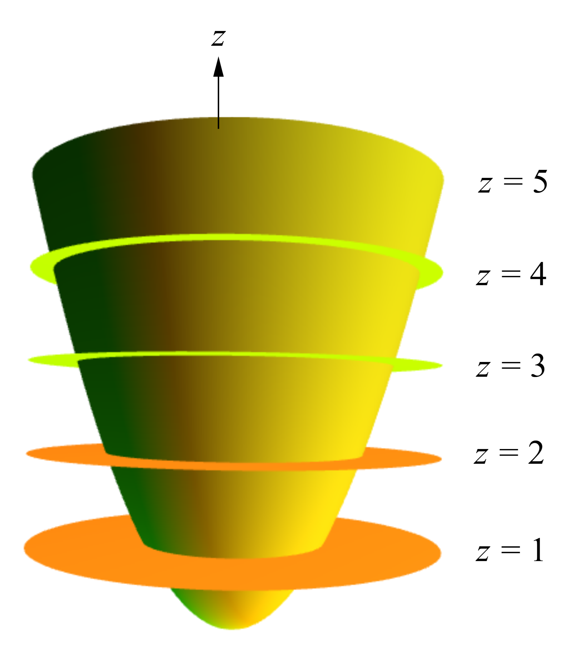
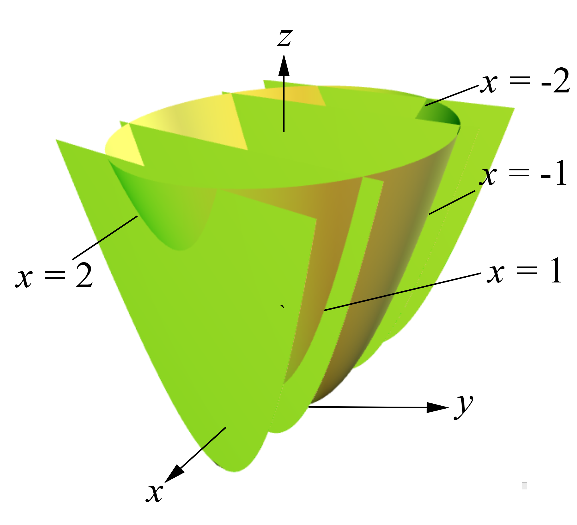
#[Vertical cross-sections][Secciones transversales verticales]#: #[Its vertical slices through the $z$-axis are all the same shape becuase of the circular symmetry. For instance, the slice through the $yz$-plane is the parabola $z = y^2$ (put $x = 0$ to see why), explaining why why the surface looks like a parabola when seen end-on. Slices through planes parallel to that, through $x = \pm 1, \pm 2, ... $ are of the form $z = y^2 + {}$ constant, and so are also parabolas, as we see in the following ficure.][Sus cortes verticales a través del eje $z$ tienen la misma forma debido a la simetría circular. Por ejemplo, el corte a través del plano $xyz$ es la parábola $z = y^2$ (pongamos $x = 0$ para ver por qué), que explica por la cual la superficie parece una parábola cuando se ve de frente. Los cortes a través de planos paralelos a ese, a través de $x = \pm 1, \pm 2, ... $ tienen la forma $z = y^2 + {}$ constante, por lo que también son parábolas, como vemos en la siguiente figura.]#

#[Practice: Reading a graph][Práctica: lectura de gráficas.l]#

Now try the exercises in Section 15.1 in Finite Mathematics and Applied Calculus. or check o see if new tutorials have been added for this chapter.